Chapter 11: Introduction to the DPLYR Package

The DPLYR package is the preeminent tool for data wrangling in R (and perhaps, in data science more generally). It provides users with an intuitive vocabulary for executing data management and analysis tasks. Learning this package will undoubtedly make your data preparation and management process faster and easier to understand.

Helpful links:

11.1 A Grammar of Data Manipulation

Hadley Wickham, the creator of the dplyr package, fittingly refers to it as a Grammar of Data Manipulation. The package provides a set of verbs to execute common data preparation tasks. One of the core challenge in programming is mapping from questions about a dataset to specific programming operations. The presence of a data manipulation grammar makes this process smoother, as it enables us to use the same vocabulary to both ask questions and execute our program. More specifically, it allows us to:

select specific columns of interest
filter down the rows
mutate a dataset to add more columns
arrange your rows in a particular order
summarise columns of interest
distinct - select the distinct set of rows
join multiple data.frame elements together

As you know, it’s possible to implement any of these procedures with base R code – this library just makes it easier to read and write. In the next section, we’ll learn how to implement these functions to ask questions of our datasets.

To practice asking questions about datasets without dplyr, see exercise-1.

11.2 Data Frame Manipulation

Many real-world questions about a dataset boil down to isolating specific rows/columns of the data and performing a simple comparison or computation (mean, median, etc.). Making yourself comfortable with the following operations will allow you to quickly write code to ask questions of your dataset.

For each of the following dplyr functions, the first argument to the function is a data frame, followed by various other arguments. Note, inside of the dplyr function parenthases, you should reference data frame columns without quotation marks (see examples below). This design choice makes the code easier to write and read, though occasionally can create challenges. To learn more, see the section below on Non-standard Evaluation.

The images in this section come from the RStudio STRATA NYC Materials, which was presented by Nathan Stephens. Exercises 4, 5, and 6 inspired by the RStudio documentation.

11.2.1 Select

The select operation allows you to choose the columns of interest out of your data frame.

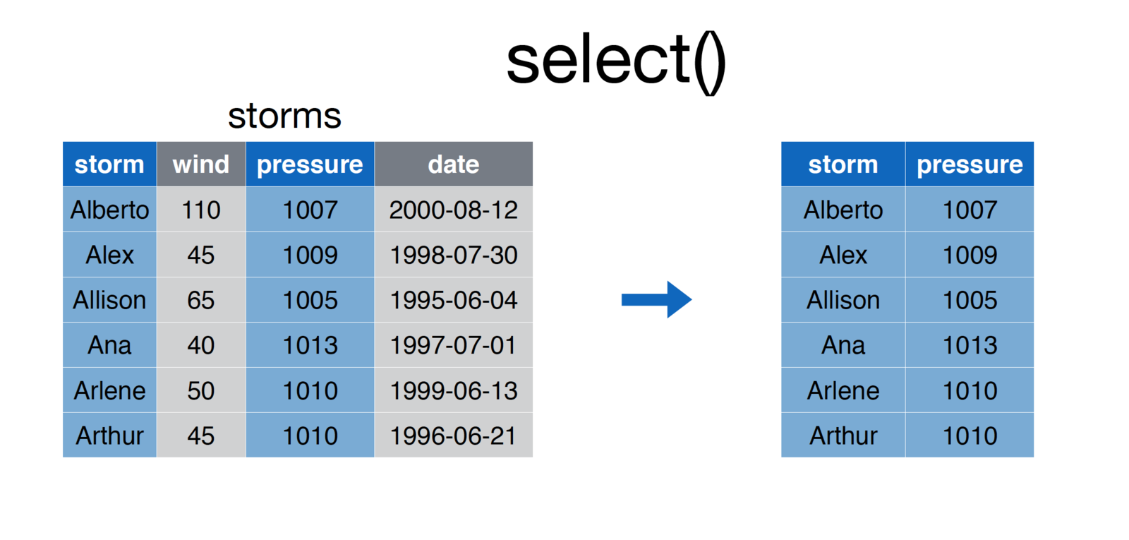
screenshot of the select function

To execute the select function, simply pass in the data frame, and the names of the columns you wish to select:

# Select `storm` and `pressure` columns from `storms` data frame
storms <- select(storms, storm, pressure)

11.2.2 Filter

Whereas select allows you to focus in on columns of interest, the filter function allows you to hone in on rows of interest. For example:

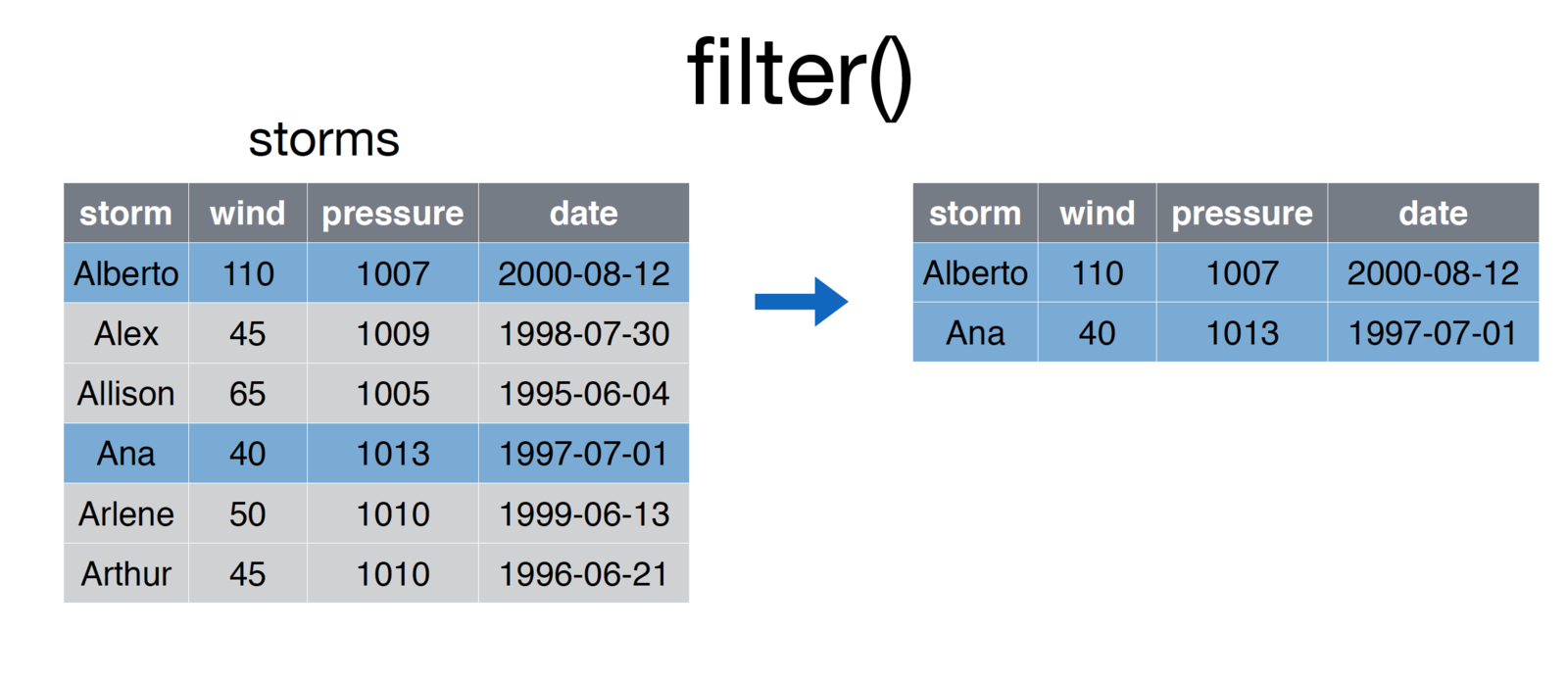
screenshot of the filter function

# Select storms whose `storm` column is in the vector ['Ana', 'Alberto']
some.storms <- filter(storms, storm %in% c('Ana', 'Alberto')

After passing in a data frame as the first argument of the function, you may specify a series of comma-separated conditions:

# Generic form of the `filter` function
filtered.rows <- filter(DATAFRAME, CONDITION-1, CONDITION-2, ..., CONDITION-N)

R will return all rows that match all condition. This is similar to saying that you want to filter down a dataframe to only the rows that meet condition-1 and condition-2.

11.2.3 Mutate

The mutate function allows you to create additional columns for your data frame:

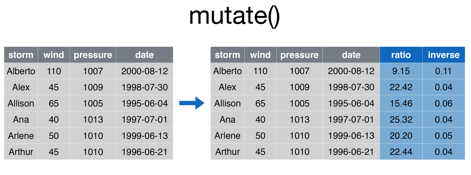
screenshot of the mutate function

# Add ratio and inverse ratio columns
storms <- mutate(storms, ratio = pressure/wind, inverse = 1/ratio

As always, the first argument to the function is that data frame with which you are working. Each additional argument is a statement that creates a new column using the following syntax:

# Generic form of the `mutate` function
more.columns <- mutate(DATAFRAME, new.column1 = old.column * 2, new.column2 = old.column * 3 )

In cases where you creating multiple variables (and therefore writing really long lines of code), you should break the single statement into multiple lines.

# Generic form of the `mutate` function
more.columns <- mutate(DATAFRAME,
                       new.column1 = old.column * 2,
                       new.column2 = old.column * 3,
                       new.column3 = old.column * 4
                      )

11.2.4 Arrange

The arrange function is what you may think of as sorting rows.

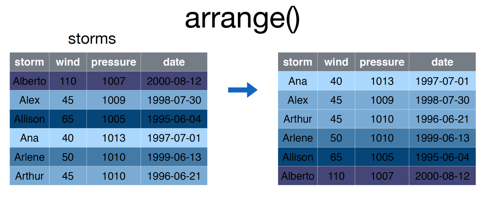
screenshot of the arrange function

# Arrange storms by increasing order of the `wind` column
storms <- arrange(storms, wind)

To sort by the reverse order of a column, simply place a minus sign (-) preceeding the varaible name. As you might imagine, you can pass multiple arguments into the arrange function to sort first by argument-1, then by argument-2.

11.2.5 Summarise

The summarise function (summarize is also accepted) creates a summary of a column, computing a single value from multipe values. The summarise function is particularly useful for grouped operations (see below), however can be used in non-grouped operations as well, for example:

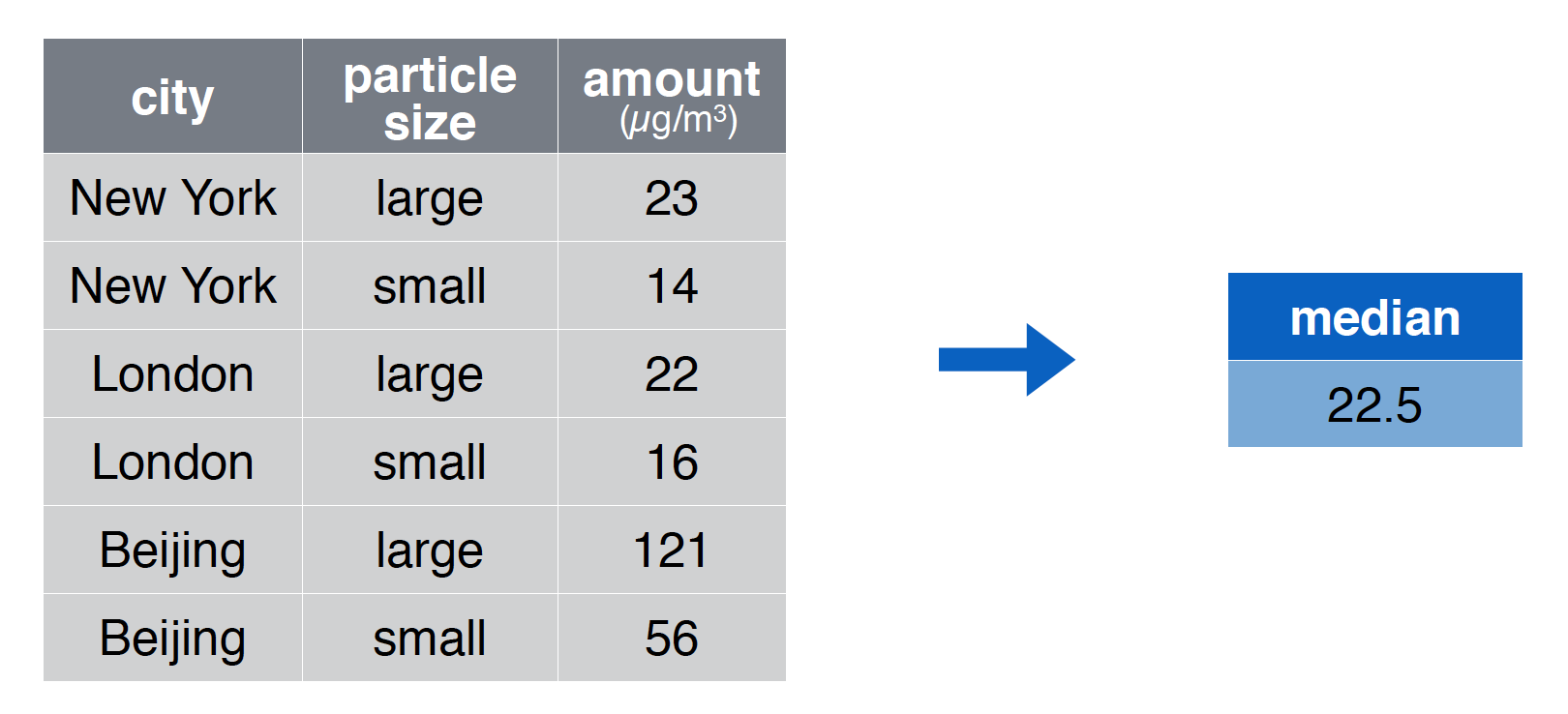
screenshot of the summarise function

# Compute the median value of the `amount` column
summary <- summarise(pollution, median = median(amount))

Each argument following the name of your data frame is a new value that will be computed using your columns. As you likely guessed, you can computed multiple summaries in the same statement:

# Compute the median value of the `amount` column
summaries <- summarise(pollution,
                       median = median(amount),
                       mean = mean(amount),
                       sum = sum(amount),
                       count = n() # nifty trick for number of observations
                       )

11.2.6 Distinct

The distinct function allows you to extract only the distinct rows in a table, evaluated based on the columns provided as arguments to the function. For example:

# Create a quick data frame
x <- c(1, 1, 2, 2, 3, 3, 4, 4)
y <- 1:8
my.df <- data.frame(x, y)

# Select distinct rows, judging by the `x` column
distinct.rows <- distinct(my.df, x)

# Select distinct rows, judging by the `x` and `y`columns
distinct.rows <- distinct(my.df, x, y)

While this is a simple way to get a unique set of rows, be careful not to unintentionally remove rows of your data which may be important.

To practice asking questions about datasets with dplyr, see exercise-2. For a more involved example, see exercise-4.

11.3 Pipe Operator

You’ve likely encountered a number of instances in which you want to take the results from one function and pass them into another function. Our approach thus far has often been to create temporary variables for use in our analysis. For example, if you’re using the mtcars dataset, you may want to ask a simple question like,

Which 4-cylinder car gets the best milage per gallon?

This simple question actually requires a few steps:

Filter down the dataset to only 4 cylinder cars
Of the 4 cylinder cars, filter down to the one with the highest mpg
Select the car name of the car from step 2.

You could then implement each step as follows:

# Add a column that is the car name
mtcars.named <- mutate(mtcars, car.name = row.names(mtcars))

# Filter down to only four cylinder cars
four.cyl <- filter(mtcars.named, cyl == 4)

# Get the best four cylinder car
best.four.cyl <- filter(four.cyl, mpg == max(mpg))

# Get the name of the car
best.car.name <- select(best.four.cyl, car.name)

While this works, it takes more lines of code than it should, and clutters our work environment with variables we won’t need to use again.

11.3.1 Nested Operations

An alternative to writing multiple lines of code is to write the desired statements nested within other statements. For example, we could write the statement above as follows:

# Add a column that is the car name
mtcars.named <- mutate(mtcars, car.name = row.names(mtcars))

# Write a nested operation to return the best car name

# Select name from the filtered data
best.car.name <- select(
                  # Filter the 4 cylinder data down by MPG
                  filter(
                    # Filter down to 4 cylinders
                    filter(
                      mtcars.named,
                      cyl == 4
                    ),
                    mpg == max(mpg)
                  ), car.name
                )

The above statement executes without creating undesirable temporary variables, but even with only 3 steps it gets quite complicated to read (think about it from the inside out for clarity). This will obviously become undecipherable for more involved operations. Luckily, the pipe operator will provide us with a more clean (and cleaver) way of achieving the above task.

11.3.2 Pipe Operator Syntax

The pipe operator provides us with a syntax for taking the results from one function and passing them in as the first argument to a second function. This avoids creating unneeded variables without the density of a nested statement. Unfortunately, the pipe operator syntax (%>%) takes getting used to. To save time, use the RStudio keyboard shortcut (cmd + shift + m)

# Add a column that is the car name
mtcars.named <- mutate(mtcars, car.name = row.names(mtcars))

# Begin your piped operation: filter down to only four cylinder cars
best.car.name <- filter(mtcars.named, cyl == 4) %>%
            filter(mpg == max(mpg)) %>%
            select(car.name)

Note, the pipe operator, which is part of the dplyr package, works with any function - not just dplyr functions. While the syntax is odd, this will completely change (simplify) the way you write code to ask questions about your data.

For an introduction to working with the pipe operator, see exercise-3.

11.4 Grouped Operations

The power of the summarise function is much clearer when we begin to group operations by rows. In the above example, we were only able to create a single summary measure for any given column, which didn’t provide much additional information. However, computing the same summary measure (mean, median, sum, etc.) by groups of rows allow you to ask more nuanced questions about your dataset. For example, if you were using the mtcars dataset, you may want to answer this question:

What is the difference in mean miles per gallon for cars with different numbers of gears (3, 4, or 5)?

This simple question requires the computation of the mean for different subsets of the data. Rather than explicitly break your data into different chunks and run the same computations, you can use the group_by function to accomplish this in a single command:

# Group cars by gear number, then compute the mean and median mpg
summary.table <- group_by(mtcars, gear) %>%
                 summarise(mean = mean(mpg), median = median(mpg), count = n())

This quickly and easily allows you to compare different subsets of your data, as diagrammed here:

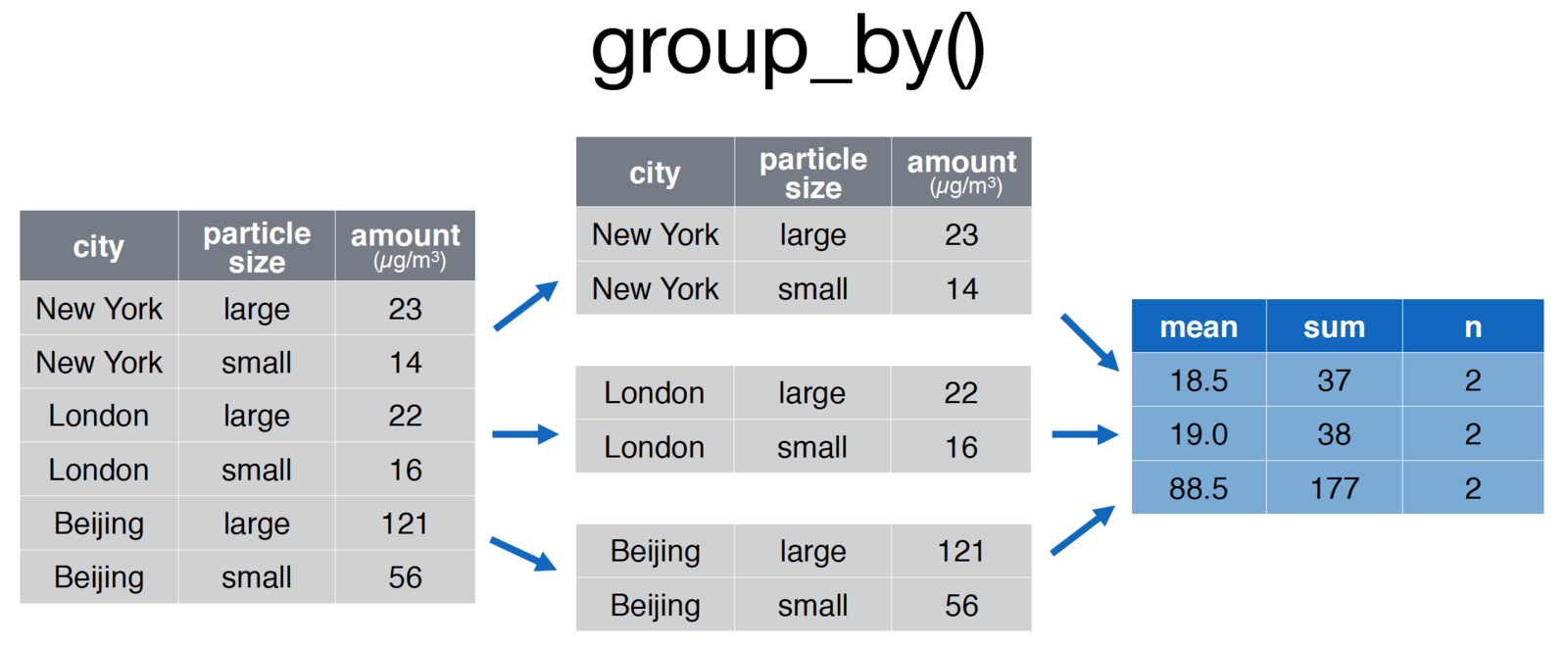
screenshot of the groupby function

# Group the pollution data.frame by city for comparison
pollution <- group_by(pollution, city) %>%
               summarise(mean = mean(amount), sum = sum(amount), n = n()
            )

For an introduction to working with grouped operations, see exercise-5.

11.5 Joins

A common procedure in the data analysis process is bringing together data from various sources, often referred to as joining or merging datasets. Joining can get quite tricky, and is a core part of understanding how to use relational databases. In this section, we’ll introduce the concept and see some simple implementations.

11.5.1 DPLYR Joins,

As stated in the documentation there are multiple families of joins in dplyr:

Mutating joins, which add new variables to one table from matching rows in another.

Filtering joins, which filter observations from one table based on whether or not they match an observation in the other table.

Set operations, which combine the observations in the data sets as if they were set elements.

(quoted directly, emphasis added).

In this section, we’ll focus on mutating joins which will add additional variables (columns) to a dataset.

First, let’s discuss the data structure: imagine you have two data frame objects, whose rows are observations and columns are information about those observations (this is how we’ve typically structured data in this course). When you join data, you are performing a matching procedure in which you have identifying columns present in both tables. Those identifiers are used to align the rows in the first table with the rows in the second table, and then the additonal information (columns from table 2) and added.

Let’s take an example where we have a table of student ids and their major. In a separate table, we have the contact information of those students (your institution very well may store this information in separate tables for privacy or organizational reasons).

# Table of contact information
student.contact <- data.frame(
    student.id=c(1, 2, 3, 4),
    email=c("id1@school.edu", "id2@school.edu", "id3@school.edu", "id4@school.ed")
)

# Table of information about majors
student.majors <- data.frame(
  student.id=c(1, 2, 3),
  major=c('sociology', 'math', 'biology')
)

To join these tables together, you could perform a left_join, which would return all of the rows in the first table, and all of the columns in the first and second table.

# Join tables by the student.id column
merged.data <- left_join(student.contact, student.majors)

This operation created a major column in the merged.data variable. Note, the order matters in the left_join statement. If you switch the order of the tables in a left_join, you will not retain observations (rows) in the second table that are not present in the first table.

# Join tables by the student.id column
merged.data <- left_join(student.majors, student.contact)

As described in the documentation, there are various joins supported by dplyr, including:

left_join: All observations in first data frame are returned

inner_join: Only observations present in both data frames are returned

full_join: All observations in both datasets are returned

right_join: Opposite of a left_join: only observations in the second data frame are returned

For an introduction to working with joins, see exercise-6. ## Non-standard Evaluation One of the features that makes dplyr such a clean and attractive way to write code is it’s use of non-standard evaluation. Inside of each dplyr function, we’ve been using variable names without quotes because the package leverages non-standard evaluation in it’s definition. Most of the time, this is not an issue. However, you’ll likely run into a situation in which you want to (or need to) use quoted values inside of your dplyr functions.

The syntax for doing this is quite easy: simply add an underscore (_) after your dplyr function, and then quote your argument values:

# Use non-standard evaluation to execute function:
mpg <- select_(mtcars, 'mpg')

# Pass in a quoted equation
mean.mpg <- summarise_(mtcars, 'mean(mpg)')

A fairly common use-case for this is if you’re storing the name of a variable of interest in a variable:

# Which variable you're interested in
var.of.interest <- 'mpg'

# Use non-standard evaluation to execute function:
mpg <- select_(mtcars, var.of.interest)